블로그 이미지
Flying Mr.Cheon youGom

Recent Comment»

Recent Post»

Recent Trackback»

« 2024/5 »
1 2 3 4
5 6 7 8 9 10 11
12 13 14 15 16 17 18
19 20 21 22 23 24 25
26 27 28 29 30 31


코로나-19 시도별 발생 현황표 - 시도명, 전일대비 확진환자 증감(합계, 해외유입, 지역발생), 확진환자수(명) (확진환자, 격리중, 격리해제, 사망자수, 발생률) 으로 구성
시도명 전일대비
확진환자 증감
확진환자 (명)
합계 해외
유입
지역
발생
확진
환자
격리
격리
해제
사망자 발생률
(*)
합계 27 5 22 11,018 937 9,821 260 21.25
서울 14 0 14 725 152 569 4 7.45
부산 0 0 0 144 14 127 3 4.22
대구 3 0 3 6,868 323 6,366 179 281.88
인천 5 1 4 124 39 85 0 4.19
광주 0 0 0 30 0 30 0 2.06
대전 0 0 0 43 3 39 1 2.92
울산 0 0 0 45 5 39 1 3.92
세종 0 0 0 47 0 47 0 13.73
경기 3 2 1 717 118 583 16 5.41
강원 0 0 0 55 9 44 2 3.57
충북 0 0 0 55 12 43 0 3.44
충남 0 0 0 144 5 139 0 6.78
전북 0 0 0 20 6 14 0 1.1
전남 1 1 0 18 5 13 0 0.97
경북 0 0 0 1,368 69 1,245 54 51.38
경남 0 0 0 119 4 115 0 3.54
제주 0 0 0 14 2 12 0 2.09
검역 1 1 0 482 171 311 0 -

출처 : http://ncov.mohw.go.kr/

:
코로나-19 시도별 발생 현황표 - 시도명, 전일대비 확진환자 증감(합계, 해외유입, 지역발생), 확진환자수(명) (확진환자, 격리중, 격리해제, 사망자수, 발생률) 으로 구성
시도명 전일대비
확진환자 증감
확진환자 (명)
합계 해외
유입
지역
발생
확진
환자
격리
격리
해제
사망자 발생률
(*)
합계 29 3 26 10,991 969 9,762 260 21.20
서울 4 1 3 711 143 564 4 7.30
부산 0 0 0 144 14 127 3 4.22
대구 0 0 0 6,865 337 6,349 179 281.76
인천 12 0 12 119 34 85 0 4.03
광주 0 0 0 30 0 30 0 2.06
대전 0 0 0 43 3 39 1 2.92
울산 0 0 0 45 3 41 1 3.92
세종 0 0 0 47 1 46 0 13.73
경기 6 0 6 714 121 577 16 5.39
강원 1 0 1 55 10 43 2 3.57
충북 3 0 3 55 12 43 0 3.44
충남 1 0 1 144 6 138 0 6.78
전북 0 0 0 20 6 14 0 1.10
전남 1 1 0 17 4 13 0 0.91
경북 1 1 0 1,368 77 1,237 54 51.38
경남 0 0 0 119 5 114 0 3.54
제주 0 0 0 14 2 12 0 2.09
검역 0 0 0 481 191 290 0 -

출처 : http://ncov.mohw.go.kr/

:
코로나-19 시도별 발생 현황표 - 시도명, 전일대비 확진환자 증감(합계, 해외유입, 지역발생), 확진환자수(명) (확진환자, 격리중, 격리해제, 사망자수, 발생률) 으로 구성
시도명 전일대비
확진환자 증감
확진환자 (명)
합계 해외
유입
지역
발생
확진
환자
격리
격리
해제
사망자 발생률
(*)
합계 27 5 22 10,936 1,008 9,670 258 21.09
서울 12 0 12 695 139 554 2 7.14
부산 0 0 0 141 13 125 3 4.13
대구 1 0 1 6,862 352 6,331 179 281.63
인천 1 0 1 105 23 82 0 3.55
광주 0 0 0 30 0 30 0 2.06
대전 2 2 0 43 4 38 1 2.92
울산 0 0 0 44 3 40 1 3.84
세종 0 0 0 47 2 45 0 13.73
경기 8 0 8 706 131 559 16 5.33
강원 0 0 0 54 11 41 2 3.51
충북 0 0 0 52 10 42 0 3.25
충남 0 0 0 143 7 136 0 6.74
전북 0 0 0 19 5 14 0 1.05
전남 0 0 0 16 4 12 0 0.86
경북 1 1 0 1,367 83 1,230 54 51.34
경남 1 1 0 118 6 112 0 3.51
제주 0 0 0 14 2 12 0 2.09
검역 1 1 0 480 213 267 0 -


출처 : http://ncov.mohw.go.kr/

:

die 2.0.5 detect it easy

보안/기술 정보 | 2020. 5. 8. 14:30 | Posted by youGom
:

keras.layers.Flatten() 

이 함수를 활용하면 된다.

model.summary()를 통해 확인해보면, input shape와 output shape가 동일하게 나오는게 보이는데,

별도 옵션이나 함수에서 output shape를 변경하는 건 없다.


Flatten() 의 역할은 n dimension을 직렬화시켜버린다. Flatten()을 통해 shape을 단순화시키고,

최종 값을 낼지, 추가 학습 모델을 넣을지 선택하면 된다.


stackoverflow에 대략 적인 답이 있어서, 이 내용을 참고 했다.

그리고 stackoverflow 뿐만 아니라, flatten()에 대한 내용은 tutorial이나 책에도 항상 나오고 있지만,

본인이 코드 작성하다보면, 실수나 생각나지 않을 수 있어서 메모해둔다.


참조 : https://github.com/keras-team/keras/issues/6351

내 코드에서 발생한 에러코드

expected ... to have 3 dimensions, but got array with shape ...


:

딥러닝을 위한 고급도구

데이터사이언스/Keras로 | 2020. 5. 7. 15:18 | Posted by youGom


7.1 Sequential 모델을 넘어서: 케라스의 함수형 API

 
Sequential


input
output
Sequential 모델: 차례대로 쌓은 층

이 책에서는 지금까지 위의 모델을 이용해서만 문제를 해결했습니다. 이런 가정은 많은 문제에 적용할 수 있지만, 아닌 경우도 존재합니다.

일부 네트워크는 개별 입력이 여러 개 필요하거나 출력이 여러 개 필요합니다. 층을 차례대로 쌓지 않고 층 사이를 연결하여 그래프처럼 만드는 네트워크도 있습니다.

예를 들어 어떤 작업은 다양한 종류의 입력이 필요합니다. 다양한 입력 소스에서 전달된 데이터를 다른 종류의 신경망 층을 사용하여 처리하고 합칩니다. 다음과 같은 모델이 만들어질 수 있는 것입니다.


모듈 병합
가격 예측
완전 연결 데이터
RNN 모듈
컨브넷 모듈
메타데이터
텍스트 설명
사진
다중 입력 모델

또한 다중 출력 모델도 가능합니다.


소설 텍스트
텍스트 처리 모듈
장르를 위한 분류 모델
시대를 위한 회귀 모델
장르
시대
다중 출력 모델

최근에 개발된 많은 신경망 구조는 선형적이지 않은 네트워크 토폴로지가 필요합니다. 비순환 유향 그래프(DAG) 같은 네트워크 구조입니다. 인셉션 모듈을 사용하는 인셉션 계열의 네트워크가 그 예시입니다. 이 모듈은 나란히 놓인 여러개의 합성곱 층을 거쳐 하나의 텐서로 출력이 합쳐집니다.


입력
Conv2D
1 * 1, strides=2
Conv2D
1 * 1
AvgPool2D
3 * 3, strides=2
Conv2D
1 * 1
Conv2D
3 * 3, strides=2
Conv2D
3 * 3
Conv2D
3 * 3
Conv2D
3 * 3, strides=2
concatenate
output
인셉션 모듈: 나란히 놓인 합성곱 층으로 구성된 서브그래프

최근에는 모델에 잔차 연결 을 추가하는 경향도 있습니다. ResNet 계열의 네트워크들이 이런 방식을 사용하기 시작했습니다. 잔차 연결은 하위 층의 출력 텐서를 상위 층의 출력 텐서에 더해서 아래층의 표현이 네트워크 위쪽으로 흘러갈 수 있도록 합니다. 하위 층에서 학습된 정보가 데이터 처리 과정에서 손실되는 것을 방지합니다.


잔차 연결
+
잔차 연결: 하위 층의 출력을 상위 층의 특성 맵에 더한다.

여러 경우에 다중 입력 모델, 다중 출력 모델, 그래프 구조를 띈 모델이 필요하지만 Sequential 모델로는 한계가 있습니다. 이런 경우 케라스의 함수형 API 를 사용할 수 있습니다.

7.1.1 함수형 API 소개

함수형 API(functional API) 에서는 직접 텐서들의 입출력을 다룹니다. 함수처럼 층을 사용하여 텐서를 입력받고 출력합니다.

간단한 예시 코드를 이용해서 Sequential과 비교해보겠습니다.

from keras.models import Sequential, Model
from keras import layers
from keras import Input

# Sequential model
seq_model = Sequential()
seq_model.add(layers.Dense(32, activation='relu', input_shape=(64,)))
seq_model.add(layers.Dense(32, activation='relu'))
seq_model.add(layers.Dense(10, activation='softmax'))

# Functianal API
input_tensor = Input(shape=(64,))
x = layers.Dense(32, activation='relu')(input_tensor)
x = layers.Dense(32, activation='relu')(x)
output_tensor = layers.Dense(10, activation='softmax')(x)

model = Model(input_tensor, output_tensor)

위 코드에서 주의할 점은 output 텐서는 반드시 input 텐서를 반복변환하여 만들 수 있어야 한다는 점입니다. 만약 그렇지 못한 입력을 줄 경우, Runtime Error가 발생합니다. 컴파일, 훈련, 평가는 다음과 같습니다.

# 컴파일
model.compile(optimizer='rmsprop', loss='categorical_crossentropy')

import numpy as np
x_train = np.random.random((1000, 64))
y_train = np.random.random((1000, 10))

# 훈련
model.fit(x_train, y_train, epochs=10, batch_size = 128)

# 평가
score = model.evalutate(x_train, y_train)

7.1.2 다중 입력 모델

함수형 API로 간단한 다중 입력 모델을 만들어봅시다. 일반적으로 이런 모델은 입력 가지를 합치기 위해 여러 텐서를 연결할 수 있는 층을 사용합니다.

예시의 모델은 질문-응답 모델입니다. 전형적인 질문-응답 모델은 2개의 입력을 가집니다.(자연어 질문, 답변에 필요한 정보가 담긴 텍스트) 그러면 모델은 답을 출력해야 합니다. 가장 간단한 구조는 미리 정의한 어휘 사전에서 소프트맥스 함수를 통해 한 단어로 된 답을 출력하는 것입니다.


참고 텍스트
Embedding
질문
Embedding
LSTM
LSTM
Concatenate
Dense
응답
질문-응답 모델

텍스트와 질문을 벡터로 인코딩하여 독립된 입력 2개를 정의합니다. 그다음 이 벡터를 연결하고 그 위에 소프트맥스 분류기를 추가합니다.

# 코드 7-1 2개의 입력을 가진 질문-응답 모델의 함수형 API 구현하기

from keras.models import Model
from keras import layers
from keras import Input

text_vocabulary_size = 10000
question_vocabulary_size = 10000
answer_vocabulary_size = 500

# 텍스트 입력은 길이가 정해지지 않은 정수 시퀀스입니다.
# 입력 이름은 지정할 수 있습니다.
text_input = Input(shape=(None, ), dtype='int32', name='text')
embedded_text = layers.Embedding(text_vocabulary_size, 64)(text_input)
encoded_text = layers.LSTM(32)(embedded_text)

# 질문도 동일한 변환을 취합니다.
question_input = Input(shape=(None, ), dtype='int32', name='question')
embedded_question = layers.Embedding(question_vocabulary_size, 64)(question_input)
encoded_question = layers.LSTM(32)(embedded_question)

# 연결합니다.
concatenated = layers.concatenate([encoded_text, encoded_question])

# softmax 분류기를 추가합니다.
answer = layers.Dense(answer_vocabulary_size, activation='softmax')(concatenated)

# 모델 객체를 만들고 2개의 입력과 출력을 주입합니다.
model = Model([text_input, question_input], answer)
model.complie(optimizer='rmsprop',loss='categorical_crossentropy',metricss=['acc'])

이렇게 입력이 2개인 모델은 2가지 방법을 훈련할 수 있습니다.

  1. 넘파이 배열의 리스트에 주입
  2. 입력 이름과 넘파이 배열로 이루어진 딕셔너리를 모델의 입력으로 주입 (입력 이름 설정시 가능)
# 코드 7-2 다중 입력 모델에 데이터 주입하기
import numpy as np
from keras.utils import to_categorical

num_samples = 1000
max_length = 100

text = np.random.randint(1, text_vocabulary_size, size=(num_samples, max_length))
question = np.random.randint(1, question_vocabulary_size, size=(num_samples, max_length))

answers = np.random.randomint(0, answer_vocabulary_size, size=num_samples)
answers = to_categorical(answers) # 원핫 인코딩

# 1.리스트 입력 사용
model.fit([text, question], answers, epochs=10, batch_size=128)
# 2. 딕셔너리 입력을 사용하여 학습
model.fit({'text':text, 'question':question}, answers, epochs=10, batch_size=128)

7.1.3 다중 출력 모델

다중 출력 모델의 예시는 소셜 미디어에서 익명 사용자의 포스트를 받아 나이, 성별, 소득을 예측하는 것입니다. 모델은 다음과 같이 생각해볼 수 있습니다.


소설 미디어 포스트
1D 컨브넷
Dense
Dense
Dense
나이
소득
성별
3개의 출력을 가진 소셜 미디어 모델
# 코드 7-3 3개의 출력을 가진 함수형 API 구현하기

from keras import layers
from keras import Input
from keras.models import Model

vocabulary_size = 50000
num_income_groups = 10

post_input = Input(shape=(None,), dtype='int32', name='posts')
embedded_posts = layers.Embedding(vocabulary_size,256)(posts_input)
x = layers.Conv1D(128, 5, activation='relu')(embedded_posts)
x = layers.MaxPooling1D(5)(x)
x = layers.Conv1D(256, 5, activation='relu')(x)
x = layers.MaxPooling1D(5)(x)
x = layers.Conv1D(256, 5, activation='relu')(x)
x = layers.GlobalMaxPooling1D()(x)
x = layers.Dense(128, activation='relu')(x)

# 출력 층에 이름 붙이기
age_prediction  = layers.Dense(1, name='age')(x)
income_prediction = layers.Dense(num_income_groups, activation='softmax', name='income')(x)
gender_prediction = layers.Dense(1, activation='sigmoid', name='gender')(x)

model= = Model(post_input, [age_prediction, income_prediction, gender_prediction])

이런 모델을 예측하기 위해서는 네트워크 출력마다 다른 손실 함수를 지정해야 합니다. 손실 값을 합치는 가장 간단한 방법은 모두 더하는 것입니다. 케라스에서는 compile 메서드에서 리스트나 딕셔너리를 사용하여 출력마다 다른 손실을 지정할 수 있습니다. 계산된 손실 값은 전체 손실 하나로 더해지고 훈련 과정에서 최소화됩니다.

# 코드 7-4 다중 출력 모델의 컴파일 옵션: 다중 손실

# 1. 리스트로 손실함수 지정
model.compile(optimizer='rmsprop', loss=['mse','categorical_crossentropy', 'binary_crossentroypy'])

# 2. 딕셔너리로 손실함수 지정
model.compile(optimizer='rmsprop', loss={'age':'mse', 'income':'categorical_crossentropy', 'gender':'binary_crossentroypy'})

하지만 단순한 합으로 하게 될 경우, 개별 손실이 가장 큰 작업 기준으로 최적화가 진행되기에 특정 값의 결과가 매우 부정확 해질 수 있습니다. 이를 해결하기 위해 가중치를 설정할 수 있습니다.

# 코드 7-5 다중 출력 모델의 컴파일 옵션: 손실 가중치
# 1. 리스트로 손실함수 지정 + 가중치
model.compile(optimizer='rmsprop', loss=['mse','categorical_crossentropy', 'binary_crossentroypy'], loss_weights=[0.25, 1., 10.])

# 2. 딕셔너리로 손실함수 지정 + 가중치
model.compile(optimizer='rmsprop', loss={'age':'mse', 'income':'categorical_crossentropy', 'gender':'binary_crossentroypy'}, loss_weights={'age':0.25, 'income':1., 'gender':10.})

다중 입력과 마찬가지로 입력 전달은 두 가지 방법으로 할 수 있습니다.

# 코드 7-6 다중 출력 모델에 데이터 주입하기

# 1. 리스트
model.fit(posts, [age_targets, income_targets, gender_targets], epochs=10, batch_size=64)

# 2. 딕셔너리
model.fit(posts, {'age' : age_targets, 'incomde' : income_targets, 'gender' : gender_targets}, epochs=10, batch_size=64)

7.1.4 층으로 구성된 비순향 유향 그래프

함수형 API는 내부 토폴로지가 복잡한 네트워크도 만들 수 있습니다. DAG에서 말이죠. 순환은 불가능합니다. 만들 수 있는 루프는 순환 층 내부에 있는 것만 가능합니다.

그래프로 구현된 몇 개의 신경망 컴포넌트가 널리 사용됩니다. 가장 유명한 2개가 앞서 언급한 인셉션 모듈과 잔차 연결입니다.

인셉션 모듈

인셉션 은 합성곱 신경망에서 인기 있는 네트워크 구조입니다. network-in-network 구조에 영감을 받은 구글러들이 만들었습니다. 가장 기본적인 인셉션 모듈 형태는 3~4개의 가지를 가집니다. 1by1 합성곱에서 3by3 합성곱이 뒤따르고 마지막에 전체 출력 특성이 합쳐집니다. 이런 구성은 네트워크가 따로따로 공간 특성과 채널 방향의 특성을 학습하도록 돕습니다. 한꺼번에 합성하는 것보다 효과가 좋습니다.

위에서 flowchart로 나타낸 모델은 인셉션V3로 케라스에서는 keras.applications.inception_v3.InceptionV3에 준비되어 있으며, ImageNet에서 사전 훈련된 가중치를 포함하고 있습니다. 이와 비슷한 엑셉션 모델도 케라스에 포함되어 있습니다. 이 합성곱 구조는 채널 방향의 학습과 공간 방향의 학습을 극단적으로 분리한다는 아이디어에 착안하여 인셉션 모듈을 깊이별 분리 합성곱으로 바꿉니다. 이 합성곱은 깊이별 합성곱 다음에 점별 합성곱이 뒤따릅니다. 인셉션 모듈의 극한 형태로 공간 특성과 채널 방향 특성을 완전히 분리합니다. 엑셉션은 인셉션V3와 거의 동일한 개수의 모델 파라미터를 가지지만 실행 속도가 더 빠르고 대규모 데이터셋에서 정확도가 더 높습니다. (효율적 사용)

잔차 연결

잔차 연결residual connection) 은 엑셉션을 포함하여 2015년 이후 등장한 많은 네트워크 구조에 있는 그래프 형태의 네트워크 컴포넌트입니다. 대규모 딥러닝 모델에서 흔히 나타나는 두 가지 문제인 그래디언트 소실과 표현 병목(representational bottleneck)을 해결했습니다. 일반적으로 10개 층 이상을 가진 모델에 잔차 연결을 추가하면 도움이 됩니다.

잔차 연결은 하위 층의 출력을 상위 층의 입력으로 사용합니다. 순서대로 놓인 네트워크를 질러가는 연결이 만들어집니다. 하위 층의 출력이 상위 층의 출력에 연결되는 것이 아니라 더해집니다. 따라서 두 출력의 크기가 동일해야 합니다. 크기가 다르면 선형 변환을 사용하여 하위 층의 활성화 출력을 목표 크기로 변환합니다.

7.1.5 층 가중치 공유

함수형 API의 중요한 또 하나의 기능은 층 객체를 여러 번 재사용할 수 있다는 것입니다. 층 객체를 두 번 호출하면 새로운 객체를 만들지 않고 각 호출에 동일한 가중치를 재사용합니다. 이런 기능 때문에 공유 가지를 가진 모델을 만들 수 있습니다.

7.1.6 층과 모델

함수형 API에서는 모델을 층처럼 사용할 수 있습니다. Sequential 클래스와 Model 클래스에서 모두 동일합니다.

7.1.7 정리

생략

7.2 케라스 콜백과 텐서보드를 사용한 딥러닝 모델 검사와 모니터링

model.fit()이나 model.fit_generator을 사용하면 실행과 동시에 결과는 제어할 방법이 없습니다. 이 절에서는 위 함수의 호출을 스스로 판단하고 동적으로 결정하는 방법을 살펴봅니다.

7.2.1 콜백을 사용하여 모델의 훈련 과정 제어하기

1장부터 6장까지 예제들을 진행하면서 가장 의문인 점은 ‘왜 과대적합이 되고난 후에도 에포크를 훈련하는가’ 였습니다. 심지어 최적의 에포크 횟수로 처음부터 새로운 훈련을 시작했습니다. 이런 방법은 낭비가 많습니다.

더 좋은 방법은 검증 손실을 관측하여 더 이상 향상되지 않는 지점에서 훈련을 멈추는 것입니다. 이를 케라스의 콜백을 이용해서 구현할 수 있습니다. 콜백(callback) 은 모델의 fit() 메서드가 호출된 때 전달되는 객체입니다. 훈련하는 동안 모델은 여러 지점에서 콜백을 호출합니다. 콜백은 모델의 상태와 성능에 대한 모든 정보에 접근하고 훈련 중지, 모델 저장, 가중치 적재 또는 모델 상태 변경 등을 처리할 수 있습니다. 다음의 사례들에서 사용할 수 있습니다.

  • 모델 체크포인트 저장 : 훈련하는 동안 어떤 지점에서 모델의 현재 가중치를 저장합니다.
  • 조기 종료(early stopping) : 검증 손실이 더 이상 향상되지 않을 때 훈련을 중지합니다.
  • 훈련하는 동안 하이퍼파라미터 값을 동적으로 조정합니다. : 옵티마이저의 학습률 같은 경우입니다.
  • 훈련과 검증 지표를 로그에 기록하거나 모델이 학습한 표현이 업데이트될 때마다 시각화합니다. : 진행 표시줄이 하나의 콜백입니다.

이제 이 예들을 살펴보겠습니다.

ModelCheckpoint와 EarlyStopping 콜백

EarlyStopping 콜백을 사용하면 정해진 에포크 동안 모니터링 지표가 향상되지 않을 때 훈련을 중지할 수 있습니다. 예를 들면 과대적합 등에서 사용할 수 있습니다. 일반적으로 이 콜백은 훈련하는 동안 모델을 계속 저장해주는 ModelCheckpoint와 함께 사용합니다. (지금까지 가장 좋은 모델만 저장가능)

import keras

# fit() 메서드의 callbacks 매개변수를 사용하여 원하는 개수만큼 콜백을 모델로 전달
callback_list = [
  keras.callbacks.EarlyStopping(
    monitor='val_acc', # 모델의 검증 정확도 모니터링
    patience=1, # 1 에포크보다 더 길게 향상되지 않으면 중단
  ),
  keras.callbacks.ModelCheckpoint(
    filepath='my_model.h5', # 저장
    monitor='val_loss',
    save_best_only=True, # 가장 좋은 모델
  )
]

model.compile(optimizer='rmsprop', loss='binary_crossentroypy', metrics['acc'])
model.fit(x,y, epochs=10, batch_size=32, callbacks=callback_list, validation_data=(x_val, y_val))

ReduceLRONPlateau 콜백

이 콜백을 사용하면 검증 손실이 향상되지 않을 때 학습률을 작게 할 수 있습니다. 손실 곡선이 평탄할 때 학습률을 작게 하거나 크게 하면 훈련 도중 지역 최솟값에서 효과적으로 빠져나올 수 있습니다.

callback_list = [
  keras.callbacks.ReduceLRONPlateau(
    monitor='val_acc',
    factor=0.1, # 콜백이 호출되면 학습률을 10배로 줄임
    patience=10,
  )
]

자신만의 콜백 만들기

내장 콜백에서 제공하지 않는 경우 필요에 따라 콜백을 만들 수 있습니다. 콜백은 keras.callbacks.Callback 클래스를 상속받아 구현합니다. 그다음 훈련하는 동안 호출될 여러 지점을 나타내기 위해 약속된 다음 메서드를 구현합니다.

method 설명
on_epoch_begin 각 에포크가 시작할 때 호출합니다.
on_epoch_end 각 에포크가 끝날 때 호출합니다.
on_batch_begin 각 배치 처리가 시작되기 전에 호출합니다.
on_batch_end 각 배치 처리가 끝난 후에 호출합니다.
on_train_begin 훈련이 시작될 때 호출합니다.
on_train_end 훈련이 끝날 때 호출합니다.

이 메서드들은 모두 log 매개변수와 함께 호출됩니다. 이 매개변수에는 이전 배치, 에포크에 대한 훈련과 검증 측정값이 담겨 있는 딕셔너리가 전달됩니다. 콜백은 다음 속성을 참조할 수 있습니다.

  • self.model: 콜백을 호출하는 모델 객체
  • self.validation_data: fit() 메서드에 전달된 검증 데이터

다음은 매 에포크의 끝에서 검증 세트의 첫 번째 샘플로 모델에 있는 모든 층의 활성화 출력을 계산하여 디스크에 저장하는 자작 콜백의 예입니다.

from keras
import numpy as np

class ActivationLogger(keras.callbacks.Callback):
  def set_model(self, model):
    self.model = model
    layer_output = [layer.output for layer in model.layers ]
    self.activation_model = keras.models.Model(model.input, layer_outputs)

  def on_epoch_end(self, epoch, log=None):
    if self.validation_data is None:
      raise RuntimeError('Requires validation_data.')
    validation_sample = self.validation_data[0][0:1]
    activation = self.activations_model.predict(validation_sample)
    f = open('activaions_at_epoch_' + str(epoch) + '.npz', 'wb')
    np.savez(f, activations)
    f.close()

7.2.2 텐서보드 소개: 텐서플로의 시각화 프레임워크

본 장의 예제 코드는 embeddings_data 매개변수의 에러로 실행을 하지 못했습니다. 링크에 같은 오류가 있음에도 원하는 결과를 찾지 못하였고, 이는 후에 수정하도록 하겠습니다.

이 장에서는 실험 결과를 처리하는 효율적인 도구인 텐서보드 를 소개하고자 합니다. 텐서플로로 백엔드를 설정하면 케라스 모델에서 사용가능합니다. 텐서보드의 핵심 목적은 훈련 모델의 내부에서 일어나는 모든 것을 시각적으로 모니터링할 수 있도록 돕는 것입니다. 모델의 최종 손실 외에 더 많은 정보를 모니터링하면 모델 작동에 대한 명확한 그림을 그릴 수 있고, 개선을 빠르게 할 수 있습니다. 텐서보드는 여러 가지 멋진 기능을 제공합니다. (모든 브라우저에서 작동)

  • 훈련하는 동안 측정 지표를 시각적으로 모니터링
  • 모델 구조를 시각화
  • 활성화 출력과 그래디언트의 히스토그램
  • 3D로 임베딩 표현

예시로 IMDB 감성 분석 문제를 위해 1D 컨브넷을 훈련합니다. 이번엔 빈도가 높은 2,000개 단어만 사용합니다.

# 코드 7-7 텐서보드를 사용한 텍스트 분류 모델
import keras
from keras import layers
from keras.datasets import imdb
from keras.preprocessing import sequence

max_features = 2000
max_len = 500

(x_train, y_train), (x_test, y_test) = imdb.load_data(num_words=max_features)
x_train = sequence.pad_sequences(x_train, maxlen=max_len)
x_test = sequence.pad_sequences(x_test, maxlen=max_len)

model = keras.models.Sequential()
model.add(layers.Embedding(max_features, 128, input_length=max_len, name='embed'))
model.add(layers.Conv1D(32, 7, activation='relu'))
model.add(layers.MaxPooling1D(5))
model.add(layers.Conv1D(32, 7, activation='relu'))
model.add(layers.GlobalMaxPooling1D())
model.add(layers.Dense(1))
model.summary()
model.compile(optimizer="rmsprop",loss="binary_crossentroypy",metrics=['acc'])

텐서보드 시작하기 전에 로그 파일이 저장될 디렉터리를 만들어야 합니다.

# 코드 7-8 텐서보드 로그 파일을 위한 디렉터리 생성하기
mkdir my_log_dir

텐서보드 콜백 객체와 함께 훈련을 진행합니다. 이 콜백은 지정된 디스크 위치에 로그 이벤트를 기록할 것입니다.

callbacks = [
  keras.callbacks.TensorBoard(
    log_dir='my_log_dir', # 저장될 path
    histogram_freq=1, # 1 에포크마다 활성화 출력의 히스토그램을 기록
    embeddings_freq=1, # 1 에포크마다 임베딩 데이터를 기록
  )
]
hitory = model.fit(x_train, y_train, epochs=20, batch_size=128, validation_split=0.2 callbacks=callbacks)

이제 명령행에서 콜백이 사용하는 로그 디렉터리를 지정하여 텐서보드 서버를 실행합니다. 텐서플로 설치시에 자동으로 설치됩니다.

tensorboard --logdir=my_log_dir

이 부분은 좀 더 공부해봐야곘습니다. :-(

7.2.3 정리

생략

7.3 모델의 성능을 최대로 끌어올리기

7.3.1 고급 구조 패턴

이전 절에서 본 잔차 연결 외에 알아야 할 디자인 패턴이 2개가 더 있습니다. 정규화와 깊이별 분리 합성곱입니다. 고성능 심층 컨브넷을 만들 때 유용합니다.

배치 정규화

정규화(normalization) 는 머신 러닝 모델에 주입되는 샘플들을 균일하게 만드는 광범위한 방법입니다. 이미 이전 예제에서 많이 사용한 방법이 있습니다. 평균을 빼고, 표준 편차로 나누어 분산을 1로 만듭니다.

normalized_data = (data - np.mean(data, axis=...)) / np.std((data, axis=...))

이전 예제에는 모델에 데이터를 주입하기 전에 정규화했습니다. 하지만 데이터 정규화는 네트워크에서 일어나는 모든 변환 후에도 고려되어야 합니다. Dense나 Conv2D 층에 들어가는 데이터의 평균이 0이고 분산이 1이라도 출력되는 데이터가 동일한 분포를 가질 것이라고 기대하기는 어렵습니다.

배치 정규화는 2015년에 아이오페와 세게디가 제안한 층의 한 종류입니다. 케라스는 BatchNormalization 클래스로 제공합니다. 훈련한는 동안 평균과 분산이 바뀌더라도 이에 적응하여 데이터를 정규화합니다. 훈련 과정에서 사용된 배치 데이터의 평균과 분산에 대한 지수 이동 평균을 내부에 유지합니다. (momentum 기본값 0.99)

배치 정규화의 주요 효과는 잔차 연결과 매우 흡사하게 그래디언트의 전파를 도와주는 것입니다. (입력과 출력의 분포가 유지) 그렇기에 더 깊은 네트워크를 구성할 수 있습니다. ResNet50, 인셉션 V3, 엑셉션 등이 있습니다. 다음은 사용하는 예시입니다.

# Conv2D 층
conv_model.add(layers.Conv2D(32, 3 activation='relu'))
conv_model.add(layers.BatchNormalization())
# Dense 층
dense_model.add(layers.Dense(32, activation='relu'))
dense_model.add(layers.BatchNormalization())

BatchNormalization 클래스에는 정규화할 특성 축을 지정하는 axis 매개변수가 있습니다. 이 매개변수의 기본값은 입력 텐서의 마지막 축을 나타내는 -1 입니다. (data_format"chanels_last"인 경우, "chanels_first"인 경우는 매개변수를 1로 설정)

2017년에는 배치 재정규화 라는 방법이 소개되었습니다. 정규화에 대해서 보다 recent한 논문을 주제로 포스팅해도 재밌을 것 같습니다.

깊이별 분리 합성곱

Conv2D를 대체하면서 더 가볍고 더 빨라 모델의 성능을 높일 수 있는 층을 소개합니다. 깊이별 분리 합성곱(depthwise separable convolution) 층은 입력 채널별로 따로따로 공간 방향의 합성곱을 수행합니다. (SeparableConv2D으로 사용합니다.) 그리고 점별 합성곱을 통해 출력 채널을 합칩니다. 공간 특성과 채널 방향 특성을 독립적으로 인식하여 학습하고, 모델 파라미터와 연산수를 줄여줍니다. 더 빠르고 효율적인 학습을 할 수 있습니다.

제한된 데이터로 작은 모델을 처음부터 훈련시킬 때 특히 더 중요합니다. 작은 데이터셋에서 이미지 분류 문제를 위한 가벼운 깊이별 분리 컨브넷을 만드는 예입니다.

 
깊이별합성곱


채널 분리
3 * 3 합성곱
3 * 3 합성곱
3 * 3 합성곱
합침
 
1 * 1 합성곱
 
깊이별 분리 합성곱: 깊이별 합성곱 다음에 합성곱이 뒤따른다.
from keras.models import Sequential, Model
from keras import layers

height = 64
width = 64
channels = 3
num_classes = 10

model = Sequential()
model.add(layers.SeparableConv2D(32, 3, activation='relu', input_shape=(height. width, channels,)))
model.add(layers.SeparableConv2D(64, 3, activation='relu'))
model.add(layer.MaxPooling2D(2))

model.add(layers.SeparableConv2D(64, 3, activation='relu'))
model.add(layers.SeparableConv2D(128, 3, activation='relu'))
model.add(layers.MaxPooling2D(2))

model.add(layers.SeparableConv2D(64, 3, activation='relu'))
model.add(layers.SeparableConv2D(128, 3, activation='relu'))
model.add(layers.GlobalAveragePooling2D())

model.add(layers.Dense(32, activation='relu'))
model.add(layers.Dense(num_classes, activation='softmax'))

model.compile(optimizer='rmsprop', loss='categorical_crossentropy')

대규모 모델은 엑셉션이 그 예시이다.

7.3.2 하이퍼파라미터 최적화

딥러닝 모델은 무작위 선택의 연속입니다. 층의 수, 유닛과 필터 수, 활성화 함수의 종류 등 설계자의 이유있는 랜덤한 선택의 연속입니다. 이런 구조에 관련된 파라미터를 역전파로 훈련되는 모델 파라미터와 구분하여 하이퍼파라미터(hyperparameter) 라고 합니다.

하이퍼파라미터 튜닝에 공식적인 규칙은 없습니다. 직관은 있을 수 있으나 정해를 찾을 수는 없습니다. 그렇다고 하이퍼파라미터 튜닝을 모두 사람이 하고 있을 수는 없기에 이것도 기계의 힘을 빌립니다. 가능한 결정 공간을 자동적, 조직적, 규칙적 방법으로 탐색해야합니다. 전형적인 최적화 과정은 다음과 같습니다.

  1. 일련의 하이퍼파라미터를 자동으로 선택합니다.
  2. 선택된 하이퍼파라미터로 모델을 만듭니다.
  3. 훈련 데이터에 학습하고 검증 데이터에서 최종 성능을 측정합니다.
  4. 다음으로 시도할 하이퍼파라미터를 자동으로 선택합니다.
  5. 이 과정을 반복합니다.
  6. 마지막으로 테스트 데이터에서 성능을 측정합니다.

주어진 하이퍼파라미터에서 얻은 검증 성능을 사용하여 다음 번에 시도할 하이퍼파라미터를 선택하는 알고리즘이 핵심입니다. 베이지안 최적화, 유전 알고리즘, 간단한 랜덤 탐색 등을 사용할 수 있습니다. 하지만 선택하는 것은 실로 어려운 일입니다. 비용이 너무 많이 들기 때문입니다. 그렇기에 가장 간단하게 하는 방법은 랜덤 탐색입니다.

랜덤 탐색보다 나은 방법으로는 파이썬 라이브러리인 Hyperopt, Hyperas 를 사용하는 것입니다. 아직은 조금 부족할 수 있는 도구지만 앞으로 발전될 가능성이 큽니다.

7.3.3 모델 앙상블

모델 앙상블(model ensemble) 은 여러 개 다른 모델의 예측을 합쳐 더 좋은 예측을 만드는 기법입니다. 캐글 같은 머신 러닝 경연 대회에서는 우승자들이 대규모 모델 앙상블을 사용합니다. 단일 모델보다 성능이 좋기 때문이죠.

가장 기본적인 앙상블은 추론에 나온 예측을 평균내는 방법입니다. 이제 더 나아가서는 가중치를 주고 평균을 내는 방법도 있습니다. 좋은 앙상블 가중치는 랜덤 서치나 넬더-미드 방법 같은 간단한 최적화 방법이 있습니다. 이외에도 지수 값을 평균할 수 있겠습니다.

앙상블이 잘 작동하게 만드는 핵심은 분류기의 다양성입니다. 모델이 서로 다른 방향으로 편향되어 있다면 상쇄를 통해 더 정확한 모델이 되는 것입니다.

모든 문제에 적용하지 못하지만 실전에서 잘 작동하는 한 가지 방법은 트리 기반 모델(랜덤 포레스트나 그래디언트 부스팅 트리)이나 심층 신경망을 앙상블하는 것입니다. 최근에 실전에서 매우 성공적으로 사용되는 기본 앙상블 스타일은 딥러닝과 얕은 모델을 섞은 넓고 깊은 모델입니다. 이런 모델은 심층 신경망과 많은 선형 모델을 함께 훈련합니다. 다양한 종류의 모델들을 함께 훈련하는 것은 모델 앙상블을 만드는 또 다른 방법입니다.

7.3.4 정리

생략

7.4 요약

생략


출처 : https://subinium.github.io/Keras-7/


"케라스 창시자에게 배우는 딥러닝" 에 있는 책 내용의 그림이 많이 담겨있어서 담아둠,

그런데.. 그림이 좀 깨지니.. 출처로 가서 살펴보는게 어쩌면 더 나을 수도 있음,

간단히 코드 볼때는 문제 없는 듯..


:

Visual Studio Code(이하 vscode)에서 Go 언어 개발 환경 세팅 방법을 포스팅 해봅니다.


go 플러그인 설치

Image

먼저 vscode에서 위 이미지와 같이 ‘go’ 플러그인을 설치합니다.


개발 디렉토리 설정

그리고 소스를 관리할 개발용 디렉토리를 설정합니다. 저같은 경우는 Windows에서는 C:\Workspace\vscode_go로 세팅했고, Linux에서는 /home/snowdeer/Workspace/go 아래에 설정했습니다.

그리고 GOPATH 환경 변수 설정을 해야 합니다. Windows에서는

Image

환경 변수 편집 화면에서 GOPATH 항목을 등록해주면 되고, Linux에서는 터미널에서 export 명령어를 이용하면 됩니다.

export GOPATH="/home/snowdeer/Workspace/go"

그리고 해당 디렉토리에는 각각 src, pkg, bin 이름의 하위 디렉토리를 만들어줍니다.


추가 파일 설치

이제 vscode에서 Go 프로그래밍을 위한 실행 파일들을 다운로드하고 설치하는 작업을 합니다. 위에서 만든 디렉토리의 src 폴더 아래에 main.go 파일을 작성하고 vscode에서 열어봅니다.

그러면 vscode에서 아래 이미지와 같이 필요한 파일들을 설치할 것인지를 물어볼 것입니다.

Image

그냥 Install All을 선택해서 모든 파일들을 설치하면 됩니다. 모든 파일들을 설치하는데는 약 5분 정도의 시간이 걸릴 수 있습니다.

Installing 9 tools at C:\Workspace\vscode_go\bin
  gopkgs
  go-outline
  go-symbols
  guru
  gorename
  godef
  goreturns
  golint
  dlv

Installing github.com/uudashr/gopkgs/cmd/gopkgs SUCCEEDED
Installing github.com/ramya-rao-a/go-outline SUCCEEDED
Installing github.com/acroca/go-symbols SUCCEEDED
Installing golang.org/x/tools/cmd/guru SUCCEEDED
Installing golang.org/x/tools/cmd/gorename SUCCEEDED
Installing github.com/rogpeppe/godef SUCCEEDED
Installing sourcegraph.com/sqs/goreturns SUCCEEDED
Installing github.com/golang/lint/golint SUCCEEDED
Installing github.com/derekparker/delve/cmd/dlv SUCCEEDED

All tools successfully installed. You're ready to Go :).


테스트 코드 및 실행

다음 코드로 실행 테스트를 해봅니다.

package main

import "fmt"

func main() {
	fmt.Println("Hello, snowdeer")
	fmt.Println("안녕. 스노우디어")
}

코드 작성 후

F5

키를 눌러 실행을 해봅니다. 브레이크 포인트(Break Point)를 걸고 디버깅을 해볼 수도 있습니다.

Image
출처 : 

https://snowdeer.github.io/go/2018/01/21/how-to-programming-go-using-visual-studio-code/

:

10 Minutes from pandas to Koalas on Apache Spark

서버/Python | 2020. 5. 7. 10:49 | Posted by youGom

pandas is a great tool to analyze small datasets on a single machine. When the need for bigger datasets arises, users often choose PySpark. However, the converting code from pandas to PySpark is not easy as PySpark APIs are considerably different from pandas APIs. Koalas makes the learning curve significantly easier by providing pandas-like APIs on the top of PySpark. With Koalas, users can take advantage of the benefits of PySpark with minimal efforts, and thus get to value much faster.

A number of blog posts such as Koalas: Easy Transition from pandas to Apache Spark, How Virgin Hyperloop One reduced processing time from hours to minutes with Koalas, and 10 minutes to Koalas in Koalas official docs have demonstrated the ease of conversion between pandas and Koalas. However, despite having the same APIs, there are subtleties when working in a distributed environment that may not be obvious to pandas users. In addition, only about ~70% of pandas APIs are implemented in Koalas. While the open-source community is actively implementing the remaining pandas APIs in Koalas, users would need to use PySpark to work around. Finally, Koalas also offers its own APIs such as to_spark(), DataFrame.map_in_pandas(), ks.sql(), etc. that can significantly improve user productivity.

Therefore, Koalas is not meant to completely replace the needs for learning PySpark. Instead, Koalas makes learning PySpark much easier by offering pandas-like functions. To be proficient in Koalas, users would need to understand the basics of Spark and some PySpark APIs. In fact, we find that users using Koalas and PySpark interchangeably tend to extract the most value from Koalas.

In particular, two types of users benefit the most from Koalas:

  • pandas users who want to scale out using PySpark and potentially migrate codebase to PySpark. Koalas is scalable and makes learning PySpark much easier
  • Spark users who want to leverage Koalas to become more productive. Koalas offers pandas-like functions so that users don’t have to build these functions themselves in PySpark

This blog post will not only demonstrate how easy it is to convert code written in pandas to Koalas, but also discuss the best practices of using Koalas; when you use Koalas as a drop-in replacement of pandas, how you can use PySpark to work around when the pandas APIs are not available in Koalas, and when you apply Koalas-specific APIs to improve productivity, etc. The example notebook in this blog can be found here.

Distributed and Partitioned Koalas DataFrame

Even though you can apply the same APIs in Koalas as in pandas, under the hood a Koalas DataFrame is very different from a pandas DataFrame. A Koalas DataFrame is distributed, which means the data is partitioned and computed across different workers. On the other hand, all the data in a pandas DataFrame fits in a single machine. As you will see, this difference leads to different behaviors.

Migration from pandas to Koalas

This section will describe how Koalas supports easy migration from pandas to Koalas with various code examples.

Object Creation

The packages below are customarily imported in order to use Koalas. Technically those packages like numpy or pandas are not necessary, but allow users to utilize Koalas more flexibly.

import numpy as np
import pandas as pd
import databricks.koalas as ks

A Koalas Series can be created by passing a list of values, the same way as a pandas Series. A Koalas Series can also be created by passing a pandas Series.

# Create a pandas Series
pser = pd.Series([1, 3, 5, np.nan, 6, 8]) 
# Create a Koalas Series
kser = ks.Series([1, 3, 5, np.nan, 6, 8])
# Create a Koalas Series by passing a pandas Series
kser = ks.Series(pser)
kser = ks.from_pandas(pser)

Best Practice: As shown below, Koalas does not guarantee the order of indices unlike pandas. This is because almost all operations in Koalas run in a distributed manner. You can use Series.sort_index() if you want ordered indices.

>>> pser
0    1.0
1    3.0
2    5.0
3    NaN
4    6.0
5    8.0
dtype: float64
>>> kser
3    NaN
2    5.0
1    3.0
5    8.0
0    1.0
4    6.0
Name: 0, dtype: float64
# Apply sort_index() to a Koalas series
>>> kser.sort_index() 
0    1.0
1    3.0
2    5.0
3    NaN
4    6.0
5    8.0
Name: 0, dtype: float64

A Koalas DataFrame can also be created by passing a NumPy array, the same way as a pandas DataFrame. A Koalas DataFrame has an Index unlike PySpark DataFrame. Therefore, Index of the pandas DataFrame would be preserved in the Koalas DataFrame after creating a Koalas DataFrame by passing a pandas DataFrame.

# Create a pandas DataFrame
pdf = pd.DataFrame({'A': np.random.rand(5),
                    'B': np.random.rand(5)})
# Create a Koalas DataFrame
kdf = ks.DataFrame({'A': np.random.rand(5),
                    'B': np.random.rand(5)})
# Create a Koalas DataFrame by passing a pandas DataFrame
kdf = ks.DataFrame(pdf)
kdf = ks.from_pandas(pdf)

Likewise, the order of indices can be sorted by DataFrame.sort_index().

>>> pdf
          A         B
0  0.015869  0.584455
1  0.224340  0.632132
2  0.637126  0.820495
3  0.810577  0.388611
4  0.037077  0.876712
>>> kdf.sort_index()
          A         B
0  0.015869  0.584455
1  0.224340  0.632132
2  0.637126  0.820495
3  0.810577  0.388611
4  0.037077  0.876712

Viewing Data

As with a pandas DataFrame, the top rows of a Koalas DataFrame can be displayed using DataFrame.head(). Generally, a confusion can occur when converting from pandas to PySpark due to the different behavior of the head() between pandas and PySpark, but Koalas supports this in the same way as pandas by using limit() of PySpark under the hood.

>>> kdf.head(2)
          A         B
0  0.015869  0.584455
1  0.224340  0.632132

A quick statistical summary of a Koalas DataFrame can be displayed using DataFrame.describe().

>>> kdf.describe()
              A         B
count  5.000000  5.000000
mean   0.344998  0.660481
std    0.360486  0.195485
min    0.015869  0.388611
25%    0.037077  0.584455
50%    0.224340  0.632132
75%    0.637126  0.820495
max    0.810577  0.876712

Sorting a Koalas DataFrame can be done using DataFrame.sort_values().

>>> kdf.sort_values(by='B')
          A         B
3  0.810577  0.388611
0  0.015869  0.584455
1  0.224340  0.632132
2  0.637126  0.820495
4  0.037077  0.876712

Transposing a Koalas DataFrame can be done using DataFrame.transpose().

>>> kdf.transpose()
          0         1         2         3         4
A  0.015869  0.224340  0.637126  0.810577  0.037077
B  0.584455  0.632132  0.820495  0.388611  0.876712

Best Practice: DataFrame.transpose() will fail when the number of rows is more than the value of compute.max_rows, which is set to 1000 by default. This is to prevent users from unknowingly executing expensive operations. In Koalas, you can easily reset the default compute.max_rows. See the official docs for DataFrame.transpose() for more details.

>>> from databricks.koalas.config import set_option, get_option
>>> ks.get_option('compute.max_rows')
1000
>>> ks.set_option('compute.max_rows', 2000)
>>> ks.get_option('compute.max_rows')
2000

Selecting or Accessing Data

As with a pandas DataFrame, selecting a single column from a Koalas DataFrame returns a Series.

>>> kdf['A']  # or kdf.A
0    0.015869
1    0.224340
2    0.637126
3    0.810577
4    0.037077
Name: A, dtype: float64

Selecting multiple columns from a Koalas DataFrame returns a Koalas DataFrame.

>>> kdf[['A', 'B']]
          A         B
0  0.015869  0.584455
1  0.224340  0.632132
2  0.637126  0.820495
3  0.810577  0.388611
4  0.037077  0.876712

Slicing is available for selecting rows from a Koalas DataFrame.

>>> kdf.loc[1:2]
          A         B
1  0.224340  0.632132
2  0.637126  0.820495

Slicing rows and columns is also available.

>>> kdf.iloc[:3, 1:2]
          B
0  0.584455
1  0.632132
2  0.820495

Best Practice: By default, Koalas disallows adding columns coming from different DataFrames or Series to a Koalas DataFrame as adding columns requires join operations which are generally expensive. This operation can be enabled by setting compute.ops_on_diff_frames to True. See Available options in the docs for more detail.

>>> kser = ks.Series([100, 200, 300, 400, 500], index=[0, 1, 2, 3, 4])
>>> kdf['C'] = kser


...
ValueError: Cannot combine the series or dataframe because it comes from a different dataframe. In order to allow this operation, enable 'compute.ops_on_diff_frames' option.
# Those are needed for managing options
>>> from databricks.koalas.config import set_option, reset_option
>>> set_option("compute.ops_on_diff_frames", True)
>>> kdf['C'] = kser
# Reset to default to avoid potential expensive operation in the future
>>> reset_option("compute.ops_on_diff_frames")
>>> kdf
          A         B    C
0  0.015869  0.584455  100
1  0.224340  0.632132  200
3  0.810577  0.388611  400
2  0.637126  0.820495  300
4  0.037077  0.876712  500

Applying a Python Function to Koalas DataFrame

DataFrame.apply() is a very powerful function favored by many pandas users. Koalas DataFrames also support this function.

>>> kdf.apply(np.cumsum)
          A         B     C
0  0.015869  0.584455   100
1  0.240210  1.216587   300
3  1.050786  1.605198   700
2  1.687913  2.425693  1000
4  1.724990  3.302404  1500

DataFrame.apply() also works for axis = 1 or ‘columns’ (0 or ‘index’ is the default).

>>> kdf.apply(np.cumsum, axis=1)
          A         B           C
0  0.015869  0.600324  100.600324
1  0.224340  0.856472  200.856472
3  0.810577  1.199187  401.199187
2  0.637126  1.457621  301.457621
4  0.037077  0.913788  500.913788

Also, a Python native function can be applied to a Koalas DataFrame.

>>> kdf.apply(lambda x: x ** 2)
          A         B       C
0  0.000252  0.341588   10000
1  0.050329  0.399591   40000
3  0.657035  0.151018  160000
2  0.405930  0.673212   90000
4  0.001375  0.768623  250000

Best Practice: While it works fine as it is, it is recommended to specify the return type hint for Spark’s return type internally when applying user defined functions to a Koalas DataFrame. If the return type hint is not specified, Koalas runs the function once for a small sample to infer the Spark return type which can be fairly expensive.

>>> def square(x) -> ks.Series[np.float64]:
...     return x ** 2
>>> kdf.apply(square)
          A         B         C
0  0.405930  0.673212   90000.0
1  0.001375  0.768623  250000.0
2  0.000252  0.341588   10000.0
3  0.657035  0.151018  160000.0
4  0.050329  0.399591   40000.0

Note that DataFrame.apply() in Koalas does not support global aggregations by its design. However, If the size of data is lower than compute.shortcut_limit, it might work because it uses pandas as a shortcut execution.

# Working properly since size of data <= compute.shortcut_limit (1000)
>>> ks.DataFrame({'A': range(1000)}).apply(lambda col: col.max())
A    999
Name: 0, dtype: int64
# Not working properly since size of data > compute.shortcut_limit (1000)
>>> ks.DataFrame({'A': range(1001)}).apply(lambda col: col.max())
A     165
A     580
A     331
A     497
A     829
A     414
A     746
A     663
A     912
A    1000
A     248
A      82
Name: 0, dtype: int64

Best Practice: In Koalas, compute.shortcut_limit (default = 1000) computes a specified number of rows in pandas as a shortcut when operating on a small dataset. Koalas uses the pandas API directly in some cases when the size of input data is below this threshold. Therefore, setting this limit too high could slow down the execution or even lead to out-of-memory errors. The following code example sets a higher compute.shortcut_limit, which then allows the previous code to work properly. See the Available options for more details.

>>> ks.set_option('compute.shortcut_limit', 1001)
>>> ks.DataFrame({'A': range(1001)}).apply(lambda col: col.max())
A    1000
Name: 0, dtype: int64

Grouping Data

Grouping data by columns is one of the common APIs in pandas. DataFrame.groupby() is available in Koalas as well.

>>> kdf.groupby('A').sum()
                 B    C
A                      
0.224340  0.632132  200
0.637126  0.820495  300
0.015869  0.584455  100
0.810577  0.388611  400
0.037077  0.876712  500

See also grouping data by multiple columns below.

>>> kdf.groupby(['A', 'B']).sum()
                     C
A        B            
0.224340 0.632132  200
0.015869 0.584455  100
0.037077 0.876712  500
0.810577 0.388611  400
0.637126 0.820495  300

Plotting and Visualizing Data

In pandas, DataFrame.plot is a good solution for visualizing data. It can be used in the same way in Koalas.

Note that Koalas leverages approximation for faster rendering. Therefore, the results could be slightly different when the number of data is larger than plotting.max_rows.

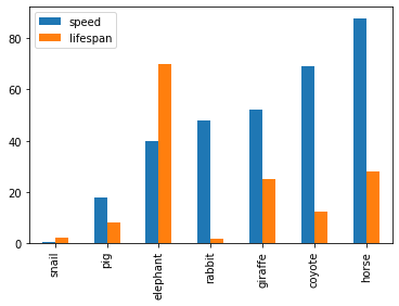
See the example below that plots a Koalas DataFrame as a bar chart with DataFrame.plot.bar().

>>> speed = [0.1, 17.5, 40, 48, 52, 69, 88]
>>> lifespan = [2, 8, 70, 1.5, 25, 12, 28]
>>> index = ['snail', 'pig', 'elephant',
...          'rabbit', 'giraffe', 'coyote', 'horse']
>>> kdf = ks.DataFrame({'speed': speed,
...                     'lifespan': lifespan}, index=index)
>>> kdf.plot.bar()

Example visualization plotting a Koalas DataFrame as a bar chart with DataFrame.plot.bar().

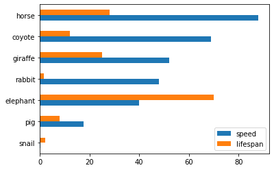
Also, The horizontal bar plot is supported with DataFrame.plot.barh()

>>> kdf.plot.barh()

Example visualization plotting a Koalas DataFrame as a horizontal bar chart

Make a pie plot using DataFrame.plot.pie().

>>> kdf = ks.DataFrame({'mass': [0.330, 4.87, 5.97],
...                     'radius': [2439.7, 6051.8, 6378.1]},
...                    index=['Mercury', 'Venus', 'Earth'])
>>> kdf.plot.pie(y='mass')

Example pie chart visualization using a Koalas DataFrame

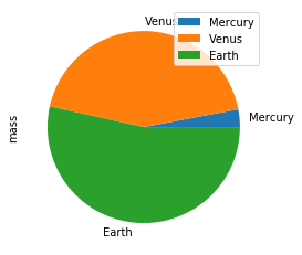
Best Practice: For bar and pie plots, only the top-n-rows are displayed to render more efficiently, which can be set by using option plotting.max_rows.

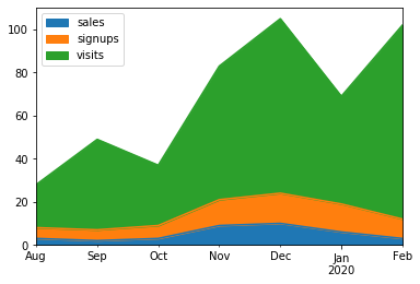
Make a stacked area plot using DataFrame.plot.area().

>>> kdf = ks.DataFrame({
...     'sales': [3, 2, 3, 9, 10, 6, 3],
...     'signups': [5, 5, 6, 12, 14, 13, 9],
...     'visits': [20, 42, 28, 62, 81, 50, 90],
... }, index=pd.date_range(start='2019/08/15', end='2020/03/09',
...                        freq='M'))
>>> kdf.plot.area()

Example stacked area plot visualization using a Koalas DataFrame

Make line charts using DataFrame.plot.line().

>>> kdf = ks.DataFrame({'pig': [20, 18, 489, 675, 1776],
...                     'horse': [4, 25, 281, 600, 1900]},
...                    index=[1990, 1997, 2003, 2009, 2014])
>>> kdf.plot.line()

Example line chart visualization using a Koalas DataFrame

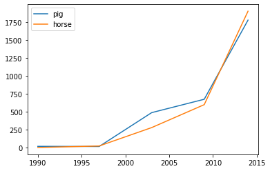
Best Practice: For area and line plots, the proportion of data that will be plotted can be set by plotting.sample_ratio. The default is 1000, or the same as plotting.max_rows. See Available options for details.

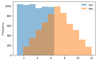
Make a histogram using DataFrame.plot.hist()

>>> kdf = pd.DataFrame(
...     np.random.randint(1, 7, 6000),
...     columns=['one'])
>>> kdf['two'] = kdf['one'] + np.random.randint(1, 7, 6000)
>>> kdf = ks.from_pandas(kdf)
>>> kdf.plot.hist(bins=12, alpha=0.5)

Example histogram visualization using a Koalas DataFrame

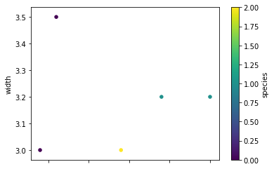
Make a scatter plot using DataFrame.plot.scatter()

>>> kdf = ks.DataFrame([[5.1, 3.5, 0], [4.9, 3.0, 0], [7.0, 3.2, 1],
...                     [6.4, 3.2, 1], [5.9, 3.0, 2]],
...                    columns=['length', 'width', 'species'])
>>> kdf.plot.scatter(x='length', y='width', c='species', colormap='viridis')

Example scatter plot visualization using a Koalas DataFrame

Missing Functionalities and Workarounds in Koalas

When working with Koalas, there are a few things to look out for. First, not all pandas APIs are currently available in Koalas. Currently, about ~70% of pandas APIs are available in Koalas. In addition, there are subtle behavioral differences between Koalas and pandas, even if the same APIs are applied. Due to the difference, it would not make sense to implement certain pandas APIs in Koalas. This section discusses common workarounds.

Using pandas APIs via Conversion

When dealing with missing pandas APIs in Koalas, a common workaround is to convert Koalas DataFrames to pandas or PySpark DataFrames, and then apply either pandas or PySpark APIs. Converting between Koalas DataFrames and pandas/PySpark DataFrames is pretty straightforward: DataFrame.to_pandas() and koalas.from_pandas() for conversion to/from pandas; DataFrame.to_spark() and DataFrame.to_koalas() for conversion to/from PySpark. However, if the Koalas DataFrame is too large to fit in one single machine, converting to pandas can cause an out-of-memory error.

Following code snippets shows a simple usage of DataFrame.to_pandas().

>>> kidx = kdf.index
>>> kidx.to_list()

...
PandasNotImplementedError: The method `pd.Index.to_list()` is not implemented. If you want to collect your data as an NumPy array, use 'to_numpy()' instead.

Best Practice: Index.to_list() raises PandasNotImplementedError. Koalas does not support this because it requires collecting all data into the client (driver node) side. A simple workaround is to convert to pandas using to_pandas().

>>> kidx.to_pandas().to_list()
[0, 1, 2, 3, 4]

Native Support for pandas Objects

Koalas has also made available the native support for pandas objects. Koalas can directly leverage pandas objects as below.

>>> kdf = ks.DataFrame({'A': 1.,
...                     'B': pd.Timestamp('20130102'),
...                     'C': pd.Series(1, index=list(range(4)), dtype='float32'),
...                     'D': np.array([3] * 4, dtype='int32'),
...                     'F': 'foo'})
>>> kdf
     A          B    C  D    F
0  1.0 2013-01-02  1.0  3  foo
1  1.0 2013-01-02  1.0  3  foo
2  1.0 2013-01-02  1.0  3  foo
3  1.0 2013-01-02  1.0  3  foo

ks.Timestamp() is not implemented yet, and ks.Series() cannot be used in the creation of Koalas DataFrame. In these cases, the pandas native objects pd.Timestamp() and pd.Series() can be used instead.

Distributing a pandas Function in Koalas

In addition, Koalas offers Koalas-specific APIs such as DataFrame.map_in_pandas(), which natively support distributing a given pandas function in Koalas.

>>> i = pd.date_range('2018-04-09', periods=2000, freq='1D1min')
>>> ts = ks.DataFrame({'A': ['timestamp']}, index=i)
>>> ts.between_time('0:15', '0:16')


...
PandasNotImplementedError: The method `pd.DataFrame.between_time()` is not implemented yet.

DataFrame.between_time() is not yet implemented in Koalas. As shown below, a simple workaround is to convert to a pandas DataFrame using to_pandas(), and then applying the function.

>>> ts.to_pandas().between_time('0:15', '0:16')
                             A
2018-04-24 00:15:00  timestamp
2018-04-25 00:16:00  timestamp
2022-04-04 00:15:00  timestamp
2022-04-05 00:16:00  timestamp

However, DataFrame.map_in_pandas() is a better alternative workaround because it does not require moving data into a single client node and potentially causing out-of-memory errors.

>>> ts.map_in_pandas(func=lambda pdf: pdf.between_time('0:15', '0:16'))
                             A
2022-04-04 00:15:00  timestamp
2022-04-05 00:16:00  timestamp
2018-04-24 00:15:00  timestamp
2018-04-25 00:16:00  timestamp

Best Practice: In this way, DataFrame.between_time(), which is a pandas function, can be performed on a distributed Koalas DataFrame because DataFrame.map_in_pandas() executes the given function across multiple nodes. See DataFrame.map_in_pandas().

Using SQL in Koalas

Koalas supports standard SQL syntax with ks.sql() which allows executing Spark SQL query and returns the result as a Koalas DataFrame.

>>> kdf = ks.DataFrame({'year': [1990, 1997, 2003, 2009, 2014],
...                     'pig': [20, 18, 489, 675, 1776],
...                     'horse': [4, 25, 281, 600, 1900]})
>>> ks.sql("SELECT * FROM {kdf} WHERE pig > 100")
   year   pig  horse
0  1990    20      4
1  1997    18     25
2  2003   489    281
3  2009   675    600
4  2014  1776   1900

Also, mixing Koalas DataFrame and pandas DataFrame is supported in a join operation.

>>> pdf = pd.DataFrame({'year': [1990, 1997, 2003, 2009, 2014],
...                     'sheep': [22, 50, 121, 445, 791],
...                     'chicken': [250, 326, 589, 1241, 2118]})
>>> ks.sql('''
...     SELECT ks.pig, pd.chicken
...     FROM {kdf} ks INNER JOIN {pdf} pd
...     ON ks.year = pd.year
...     ORDER BY ks.pig, pd.chicken''')
    pig  chicken
0    18      326
1    20      250
2   489      589
3   675     1241
4  1776     2118

Working with PySpark

You can also apply several PySpark APIs on Koalas DataFrames. PySpark background can make you more productive when working in Koalas. If you know PySpark, you can use PySpark APIs as workarounds when the pandas-equivalent APIs are not available in Koalas. If you feel comfortable with PySpark, you can use many rich features such as the Spark UI, history server, etc.

Conversion from and to PySpark DataFrame

A Koalas DataFrame can be easily converted to a PySpark DataFrame using DataFrame.to_spark(), similar to DataFrame.to_pandas(). On the other hand, a PySpark DataFrame can be easily converted to a Koalas DataFrame using DataFrame.to_koalas(), which extends the Spark DataFrame class.

>>> kdf = ks.DataFrame({'A': [1, 2, 3, 4, 5], 'B': [10, 20, 30, 40, 50]})
>>> sdf = kdf.to_spark()
>>> type(sdf)
pyspark.sql.dataframe.DataFrame
>>> sdf.show()
+---+---+
|  A|  B|
+---+---+
|  1| 10|
|  2| 20|
|  3| 30|
|  4| 40|
|  5| 50|
+---+---+

Note that converting from PySpark to Koalas can cause an out-of-memory error when the default index type is sequence. Default index type can be set by compute.default_index_type (default = sequence). If the default index must be the sequence in a large dataset, distributed-sequence should be used.

>>> from databricks.koalas import option_context
>>> with option_context(
...         "compute.default_index_type", "distributed-sequence"):
...     kdf = sdf.to_koalas()
>>> type(kdf)
databricks.koalas.frame.DataFrame
>>> kdf
   A   B
3  4  40
1  2  20
2  3  30
4  5  50
0  1  10

Best Practice: Converting from a PySpark DataFrame to Koalas DataFrame can have some overhead because it requires creating a new default index internally – PySpark DataFrames do not have indices. You can avoid this overhead by specifying the column that can be used as an index column. See the Default Index type for more detail.

>>> sdf.to_koalas(index_col='A')
    B
A    
1  10
2  20
3  30
4  40
5  50

Checking Spark’s Execution Plans

DataFrame.explain() is a useful PySpark API and is also available in Koalas. It can show the Spark execution plans before the actual execution. It helps you understand and predict the actual execution and avoid the critical performance degradation.

from databricks.koalas import option_context

with option_context(
        "compute.ops_on_diff_frames", True,
        "compute.default_index_type", 'distributed'):
    df = ks.range(10) + ks.range(10)
    df.explain()

The command above simply adds two DataFrames with the same values. The result is shown below.

== Physical Plan ==
*(5) Project [...]
+- SortMergeJoin [...], FullOuter
   :- *(2) Sort [...], false, 0
   :  +- Exchange hashpartitioning(...), [id=#]
   :     +- *(1) Project [...]
   :        +- *(1) Range (0, 10, step=1, splits=12)
   +- *(4) Sort [...], false, 0
      +- ReusedExchange [...], Exchange hashpartitioning(...), [id=#]

As shown in the physical plan, the execution will be fairly expensive because it will perform the sort merge join to combine DataFrames. To improve the execution performance, you can reuse the same DataFrame to avoid the merge. See Physical Plans in Spark SQL to learn more.

with option_context(
        "compute.ops_on_diff_frames", False,
        "compute.default_index_type", 'distributed'):
    df = ks.range(10)
    df = df + df
    df.explain()

Now it uses the same DataFrame for the operations and avoids combining different DataFrames and triggering a sort merge join, which is enabled by compute.ops_on_diff_frames.

== Physical Plan ==
*(1) Project [...]
+- *(1) Project [...]
   +- *(1) Range (0, 10, step=1, splits=12)

This operation is much cheaper than the previous one while producing the same output. Examine DataFrame.explain() to help improve your code efficiency.

Caching DataFrame

DataFrame.cache() is a useful PySpark API and is available in Koalas as well. It is used to cache the output from a Koalas operation so that it would not need to be computed again in the subsequent execution. This would significantly improve the execution speed when the output needs to be accessed repeatedly.

with option_context("compute.default_index_type", 'distributed'):
    df = ks.range(10)
    new_df = (df + df).cache()  # `(df + df)` is cached here as `df`
    new_df.explain()

As the physical plan shows below, new_df will be cached once it is executed.

== Physical Plan ==
*(1) InMemoryTableScan [...]
   +- InMemoryRelation [...], StorageLevel(...)
      +- *(1) Project [...]
         +- *(1) Project [...]
            +- *(1) Project [...]
               +- *(1) Range (0, 10, step=1, splits=12)

InMemoryTableScan and InMemoryRelation mean the new_df will be cached – it does not need to perform the same (df + df) operation when it is executed the next time.

A cached DataFrame can be uncached by DataFrame.unpersist().

new_df.unpersist()

Best Practice: A cached DataFrame can be used in a context manager to ensure the cached scope against the DataFrame. It will be cached and uncached back within the with scope.

with (df + df).cache() as df:
    df.explain()

Conclusion

The examples in this blog demonstrate how easily you can migrate your pandas codebase to Koalas when working with large datasets. Koalas is built on top of PySpark, and provides the same API interface as pandas. While there are subtle differences between pandas and Koalas, Koalas provides additional Koalas-specific functions to make it easy when working in a distributed setting. Finally, this blog shows common workarounds and best practices when working in Koalas. For pandas users who need to scale out, Koalas fits their needs nicely.

Get Started with Koalas on Apache Spark

You can get started with trying examples in this blog in this notebook, visit the Koalas documentation and peruse examples, and contribute at Koalas GitHub. Also, join the koalas-dev mailing list for discussions and new release announcements.

References

출처 : 

https://databricks.com/blog/2020/03/31/10-minutes-from-pandas-to-koalas-on-apache-spark.html


'서버 > Python' 카테고리의 다른 글

jupyter themes 주피터 노트북 테마 바꾸기  (0) 2020.06.24
couchdb basic tutorial  (0) 2020.04.26
tistory api access token 얻는 방법  (0) 2020.04.25
gsm bts using rasberry pi 3  (0) 2019.03.04
pwn basic in python  (0) 2018.12.11
:

 
공지 페이지 : 

http://www.moef.go.kr/sns/2020/emgncEcnmyMtg.do?slideCnt=03&category1=infograp#05

-----------------------------------------------------------------------------------------------------

더보기

전국민에게 100만 원(4인이상 가구 기준)을 긴급재난 지원금으로 지급합니다. 
※ 이를 위한 12.2조 원 규모의 제2회 추가경정예산이 확정되었습니다.

  • 대상확인: 5월4일(월)부터 긴급재난지원금 홈페이지에서 조회
    인터넷주소(URL): 긴급재난지원금.kr
  • 지급수단: 보유 중인 신용카드, 체크카드, 지역사랑상품권, 지자체 선불카드 중 선택
  • 신청방법: 대상가구의 세대주 신청 원칙
    - 생계급여, 기초연금, 장애인연금 수급 가구(약 270만)는 기존 복지전달체계 및 계좌정보를 활용하여 신청 없이 현금 지급
  • 지급시기: 가능한 빨리 받을 수 있도록 최대한 신속 지급
    - 계좌번호가 확보된 취약계층(약 270만가구): 5월4일(월)부터 계좌이체 - 온라인 신청: 5월11일(월) 신청 시작 → 5월13일(수)부터 지급 시작 - 방문신청 : 5월18일(월)부터 신청 접수 후 지급
  • 요일제: 혼잡 및 코로나19 확산 예방을 위해 시행 초기 요일제 추진 예정

긴급재난지원금 가구규모별 지원액

단위 : 원

구분1인가구2인가구3인가구4인 가구 이상

지원규모

400,000

600,000

800,000

1,000,000

※ 건강보험료상 가구 기준

:
코로나-19 시도별 발생 현황표 - 시도명, 전일대비 확진환자 증감(합계, 해외유입, 지역발생), 확진환자수(명) (확진환자, 격리중, 격리해제, 사망자수, 발생률) 으로 구성
시도명 전일대비
확진환자 증감
확진환자 (명)
합계 해외
유입
지역
발생
확진
환자
격리
격리
해제
사망자 발생률
(*)
합계 4 3 1 10,810 1,135 9,419 256 20.85
서울 0 0 0 637 127 508 2 6.54
부산 0 0 0 138 15 120 3 4.04
대구 0 0 0 6,856 429 6,249 178 281.39
인천 0 0 0 97 25 72 0 3.28
광주 0 0 0 30 2 28 0 2.06
대전 1 1 0 41 2 38 1 2.78
울산 0 0 0 44 6 37 1 3.84
세종 0 0 0 46 1 45 0 13.44
경기 1 0 1 682 128 538 16 5.15
강원 0 0 0 53 9 42 2 3.44
충북 1 1 0 46 4 42 0 2.88
충남 0 0 0 143 15 128 0 6.74
전북 0 0 0 18 4 14 0 0.99
전남 0 0 0 16 4 12 0 0.86
경북 0 0 0 1,366 115 1,198 53 51.31
경남 0 0 0 117 12 105 0 3.48
제주 0 0 0 13 1 12 0 1.94
검역 1 1 0 467 236 231 0 -


출처 : http://ncov.mohw.go.kr/

: